Markets operate in two different modes: random (or “normal,” in the Gaussian world) and fractal (non-normal, extreme). My work on the luck factor (i.e., a person’s sequence of returns) over 20 years has indicated that markets are random about 94% of the time and fractal for the remaining 6% (about 3% up and 3% down) of the time.
When the markets are in random mode, well-known strategies such as asset allocation, diversification, rebalancing, dollar-cost averaging, buy-and-hold, work perfectly well. But these strategies don’t help much when markets are fractally going down. You might say, why worry if it happens only 3% of the time? The answer is simple: a big drop can wipe out 10 years of retirement income.
After a fractal event, we all hope that a recovery comes quickly. Fortunately, central banks have jumped in to help. But these rescues did not come cheap. The global total debt, which was $87 trillion (U.S.) dollars in year 2000, is now an estimated $253 trillion (before accounting for the financial impact of the COVID-19 event), according to The Guardian, January 8, 2020.
Our question is this: How many months or years should it take a portfolio to recover its original value after a big drawdown (assuming that central banks keep bailing out the economy—and shifting the burden to future generations)?
In our analysis, we make projections using actual market history, which we call “aftcasting” (as opposed to “forecasting”). Within a single chart, aftcasting can display the outcomes of all historical asset values of all portfolios since 1900. That is, it offers a bird’s-eye view of all outcomes for a given client-scenario. It provides the long-term portfolio success and failure statistics with exact historical accuracy by including actual historical equity performance, inflation rates, and interest rates, as well as the actual historical sequencing/correlation of these data sets.
Keith and Jane
Let’s consider a hypothetical accumulation portfolio. Keith, 30, has a portfolio worth $100,000. The asset mix is 70% equities and 30% fixed income. For equities, we use S&P500 index as a proxy. We use the historical interest on 6-month CDs plus 0.5% as the net yield for the fixed income portion of his portfolio. This approximates a bond ladder with an average maturity of about five to seven years at current yields, assuming no defaults and no capital gains/losses.
Keith plans to add $4,000 each year to his portfolio. Thus his accumulation ratio is 4%, which expresses the annual addition as a percentage of the portfolio value ($4,000 / $100,000).
Then a fractal event happens. Keith’s portfolio loses 25% of its value, dropping to $75,000. Keith asks, “When will my portfolio be back at $100,000, the pre-crash value?”
Figure 1 displays the aftcast. In an aftcast, there are no assumed rates of return. Each of the gray lines represents future market performance, starting in each specific year since 1900. The blue line represents the median portfolio; half of the gray lines are above it and half below. The green line indicates the “lucky” outcome; it represents the top decile (top 10%) of all outcomes. A lucky outcome typically happens when a recovery is “V-shaped.” The red line indicates the “unlucky” outcome; it represents the bottom decile. An unlucky outcome usually signifies a multi-year bear market (like those beginning in 1929 or 2000) with several after-shocks.
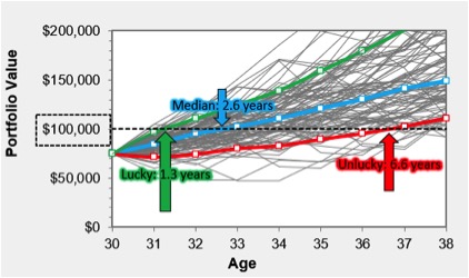
Note that it took about 2.6 years for the median line to reach the original portfolio value of $100,000 (the horizontal dashed line). If this were a V-shaped recovery, however, Keith’s portfolio would recover in about 16 months. If this were a multi-year bear market, he would not see the $100,000 mark again for 6.6 years, thanks mainly to his periodic contributions.
Our next example involves someone in the retirement stage. Jane, 65, has just retired. Her portfolio, worth $500,000, consists of 40% equities and 60% fixed income investments.
Jane needs her savings to generate an income of $15,000 each year. Her initial withdrawal rate is 3% ($15,000 / $500,000), which she can sustain indefinitely. She plans to withdraw $15,000 per year (indexed to the Consumer Price Index) or the amount of her Minimum Required Distribution from tax-deferred accounts, whichever is larger.
A fractal event happens, and Jane’s portfolio value drops 25% to $375,000. Jane asks, “When will my portfolio get back to its $500,000 pre-crash value?” Figure 2 displays the aftcast. (To simplify the illustration, the loss-percentages suffered by Jane and Keith are kept equal at 25%, even though, due to their different asset allocations, their portfolio balances would respond differently to market conditions.)
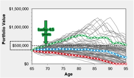
If this loss were followed by a V-shaped recovery, Jane would see her portfolio value reach the original $500,000 after about 4.5 years. The median portfolio never reaches that $500,000 mark, however.
Our question was not whether or not Jane will have lifelong income; she likely will unless she lives far beyond age 90. We asked, “When will Jane’s portfolio reach $500,000? again.” It probably won’t.
Median recovery times of different asset allocations
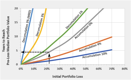
To complete this study, I ran a multitude of scenarios. The results are summarized in Figure 3. Let’s use an example to illustrate them further.
Jeff has a balanced portfolio of $1 million. He does not add any money to it, nor does he need any income from it. (His “accumulation rate” for these purposes is zero.) After an unfortunate market event, his portfolio is down 22%. When can Jeff expect to see his portfolio back at the $1 million mark?
In Figure 3, we draw a vertical line (the dashed line on the chart) starting at the 22% initial portfolio loss on the horizontal axis. Continue this line until it reaches 0% accumulation curve. From this point, draw a horizontal line towards the left axis. It’s about 4.4 years. Historically, this is how long it took the median portfolio to reach its pre-loss value.
You might wonder what would happen if, instead of following the median path, this loss were followed by a V-shaped recovery (lucky outcome) or a multi-year downturn (unlucky). For precise answers, you’d need to run an aftcast for each specific scenario. But there’s a rule of thumb.
To estimate the lucky outcome, divide the median by 3. To estimate the unlucky outcome, multiply the median by 2.5. In our example, the median was 4.4 years. If Jeff is lucky, his portfolio will bounce back to $1 million in 1.5 years, calculated as 4.4 / 3. If he is unlucky, the rebound may take as long as 11 years, calculated as 4.4 x 2.5. This assumes that Jeff stays invested throughout the volatility period and does not bail out.
You might ask about the impact of asset allocation. When fractal events happen, asset mix doesn’t greatly affect the recovery time. If the portfolio is heavy in equities, it loses more but recovers faster. The difference in asset mix impacts the dollar dimension much more than the time dimension. The important factor here is the client’s ability to stay-the-course during adverse market events. (In this article, I used 40/60 asset mix for all decumulation portfolios and 70/30 for all accumulation portfolios.)
Let’s drill-down on the problem of staying power, aka “behavioral risk.” Consider two investors, both in the early stages of investing. Both are 30 years old and have $100,000 in their portfolios. They each add $4,000 annually to their portfolio.
Chase and Grace
Chase is more aggressive; he believes that stocks are “for the long run.” He proudly holds a portfolio of 100% stocks. The only problem is, Chase never tested his own risk tolerance.
Grace, by contrast, is a conservative investor. She knows her risk tolerance and holds an asset mix of 40% stocks/60% fixed income. A fractal market event happens, and the equity index drops 40%. The fixed income portion stays the same. Now, Chase’s portfolio is worth only $60,000. Having never experienced a loss like this, he gets scared and changes his asset mix to 40/60. Grace’s portfolio is now worth $84k and she holds on to her investments.
Their experiences over the next 20 years are depicted in Figure 4. The lines show their median portfolio values based on market history since 1900. Because Grace had staying power, she accumulated more assets than Chase, who bailed out and reset his asset mix. That mistake cost him a lot of money and accumulation time.
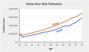
Even if Grace had gotten scared and made her asset mix more conservative, she would still be ahead of Chase, because her initial losses were lower.
The best time to make an asset mix more conservative is not after a loss but before one. The best opportunities to discover your own risk tolerance are actual life experiences. No risk tolerance questionnaire will give you an accurate answer. The lesson: Stay conservative until you discover your own risk tolerance.
In this example, we looked at only a single occurrence of bailing-out behavior. In my 24 years in the investment business, I can say with confidence that if this type of misbehavior happens once, it will likely happen again. Such self-sabotage will reoccur until the lesson is learned.
Practical action steps
To summarize the lessons of this study:
- Know thy risk tolerance. The most effective way of increasing your investment success is to look at yourself first and decide on your risk tolerance. Err on the side of less risk.
- During the early accumulation stage, keep the portfolio at a conservative 40% equity/60% fixed income. Maintain this mix until your annual accumulation dollar amount is less than 4% of the portfolio value. Regardless of how many risk tolerance questionnaires you fill out, you won’t know how you will respond to black swan events until they actually happen. Can you hang on to your investments when large, multi-year losses happen? You won’t know that until it happens for the first time. Stay conservative until then.
- During the mature accumulation stage, if your risk tolerance permits, you can maintain a 60/40 mix, which will provide sufficient growth with reasonable risk.
- Ten years before retirement, move your asset mix back to 40/60. You might need a full 10 years of recovery time after a nasty black swan event. Therefore, between ages 60 and 65, reduce the risk.
- Once you retire and switch from accumulation to decumulation, the math of loss flips on its head—dramatically so. Even if your initial withdrawal rate is a modest 3%, you may never again see the pre-loss asset value of the portfolio.
- If the withdrawal rate in retirement (3% to 4%) is too low to cover essential expenses, consider guaranteed income products such as life annuities or segregated funds (variable annuities) with guaranteed lifetime withdrawal benefits. Why? When you’re using a safe withdrawal rate, a portfolio loss as small as 15% can reduce income noticeably.
- If withdrawals from the portfolio are intended purely for discretionary and non-essential expenses, but preservation of capital is important, then use a variable annuity with a lifetime withdrawal benefit to protect assets, as well as to reduce behavioral risk.
- If withdrawals from the portfolio are for discretionary and non-essential expenses only, and preservation of capital is not important, a traditional investment portfolio will work.
This study is based on the market history of the last century. It assumes that the current central bank borrowing binge can continue indefinitely. During the last century, fixed income was the “safer” side of a portfolio. Going forward, it might turn into the riskier side. We shall see. Meanwhile, enjoy this recovery.
Jim Otar is a retired financial planner and retired professional engineer. He is the founder of www.retirementoptimizer.com. His past articles won the CFP Board Article Awards in 2001 and 2002. He is the author of Unveiling the Retirement Myth, a 525-page textbook. He can be reached at [email protected]


